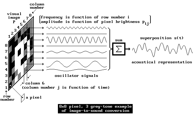
 In order to achieve a high resolution, each image is transformed into a time-multiplexed auditory representation. |
Page contents:
|
In order to achieve a high resolution, each image is transformed into a time-multiplexed auditory representation. |
Many other types of frequency distribution could be used for an auditory display. For example there is the mel-scale that stems from perceptual research on subjective equidistance perceived in frequency steps, and the bark-scale that originates in critical band measurements. These additional psychophysical scaling functions are available as options in The vOICe for Windows. An advantage of perception-based distributions is the possibility to best exploit the mix of strengths and weaknesses in auditory perception and segregation. A disadvantage shared by perception-based distributions and psychophysical scaling functions is that they easily lead to a proliferation of alternative expressions and parameter sets, each dedicated to a particular measurement procedure that more or less highlights particular perceptual limitations under a limited set of conditions. In addition, there is the risk of optimizing sonification mappings for existing psychological and cultural habits (with demographic variations) rather than for any fundamental limits that would only appear after prolonged exposure and training (learning and/or unlearning). Furthermore, there is the role of informational masking in becoming aware of relevant details in complex soundscapes, and this factor is likely very dependent on user experience. Following the intuitive mapping preferences of listeners is not necessarily the right choice for obtaining best performance results in the long run.
The following template allows you to obtain lists of frequencies and frequency steps for several types of frequency distribution, and you can override several of the default parameter settings:
|
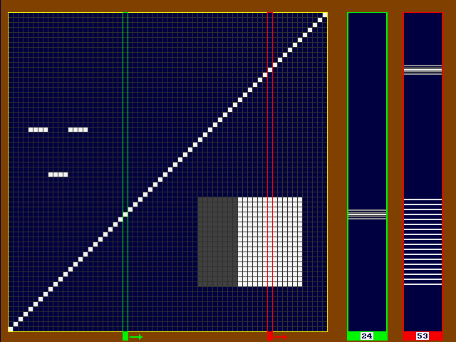
![]() For this particular auditory scene, the sound was synthesized off-line by a computer
program (ANSI C source code arti1.c, or its port to Python 3
arti1.py). The unwanted ``speckles'' in the sound are the
consequence of the simple rectangular time window employed in turning pixel sounds
on or off. Here follows an overview of several computer-generated soundscapes with
associated (completely self-contained) program sources:
For this particular auditory scene, the sound was synthesized off-line by a computer
program (ANSI C source code arti1.c, or its port to Python 3
arti1.py). The unwanted ``speckles'' in the sound are the
consequence of the simple rectangular time window employed in turning pixel sounds
on or off. Here follows an overview of several computer-generated soundscapes with
associated (completely self-contained) program sources:
|
Artificial 64 × 64 pixel / 16 grey-tone scenes
21K soundscapes (20 kHz / 8 bit / 1.05s, loop=true) |
|||
|---|---|---|---|
Lines & rectangles |
B&W drawing |
Math curve plot |
PC screen layout: icons & windows |
 |
 |
 |
 |
| More scenes | |||
Speech synthesis |
Letters A, B & C |
Parked car |
Human face |
 |
 |
 |
 |
... and for those who wish to further explore the possibilities of software-based hifi stereo soundscape generation, the source of a more elaborate computer program, hificode.c, is available. This program was written to provide you with additional options for obtaining higher quality soundscapes (in this example hificode.wav). The program can generate CD quality 44.1 kHz 16-bit stereo samples, where the stereo effect now incorporates both interaural time delays and head-masking. Furthermore, the above-mentioned speckles are avoided by using smooth quadratic (variation diminishing, or QVD) B-spline time windows which completely remove the column switching discontinuities. Finally, a variation of the hificode.c program for live camera processing with OpenCV on Windows or Linux is available as hificode_OpenCV.cpp (or its direct port to Python 3 hificode_OpenCV.py, which in a Python interpreter tends to run too slowly for practical use). A zipped Microsoft Visual Studio 2010 project for hificode_OpenCV.cpp is vOICeOpenCV.zip, in which you will likely need to adapt the following Project properties to account for your version of OpenCV (here 2.4.11) and the path where you installed it: C/C++ | Additional Include Directories, Linker | Additional Library Directories, Linker | Input | Additional Dependencies.
 Please note that the software in this section has not been optimized for speed, code quality or any other
purpose but to provide a crude but functional reference for use in implementation and testing on various platforms.
You may use the software (source code) that is directly linked from this section on this (and only this) web page under the Creative Commons Attribution 4.0 International License (CC BY 4.0): that is, you may freely share and adapt the software for any purpose, including commercial usage, provided that in all places where you describe or use the functionality you give credit to the author (Copyright © Peter B.L. Meijer) for providing the original version of the software, and include a link back to this web page (http://www.seeingwithsound.com/im2sound.htm)
and/or website (http://www.seeingwithsound.com).
Please note that the software in this section has not been optimized for speed, code quality or any other
purpose but to provide a crude but functional reference for use in implementation and testing on various platforms.
You may use the software (source code) that is directly linked from this section on this (and only this) web page under the Creative Commons Attribution 4.0 International License (CC BY 4.0): that is, you may freely share and adapt the software for any purpose, including commercial usage, provided that in all places where you describe or use the functionality you give credit to the author (Copyright © Peter B.L. Meijer) for providing the original version of the software, and include a link back to this web page (http://www.seeingwithsound.com/im2sound.htm)
and/or website (http://www.seeingwithsound.com).
Note: instead of implementing The vOICe image-to-sound mapping algorithms in python, you can also simply launch
The vOICe web app from within python using just a few lines of code:Thanks to the persistent caching of progressive web apps, you need to be online only once when running this code, and in subsequent runs it will work offline as well. |
In graphical user interfaces (GUI's), icons displayed on a computer screen would become simple earcons when using bright icons on a dark background. For specific applications like these, there may always exist more appropriate but less general image to sound mappings. For instance, one could attach fixed or parameterized earcons to the small collection of object types that make up a GUI - widgets of several categories like the button, the checkbox, the menu, the scrollbar, the dialog, and, of course, the window. However, the abstract mapping of The vOICe is far more general by covering arbitrary images. This is now also demonstrated by The vOICe Java applet and by The vOICe for Windows.
Links to related online material available at other sites can be found in the external links page, and projects in which image-tosound mappings similar to or related to The vOICe mapping are employed can be found on the related projects page.
![]()
|
|
| Apart from sonifying natural images and figurative drawings, one could also use or superimpose any computer-generated artificial images, or spectrographic images derived from natural sounds, as input for The vOICe mapping. Thereby, one could indeed cover a very wide range of sound types, ranging from human speech or fixed auditory icons up to parameterized earcons involving melodic or rhythmic motives. The drawback would be that much additional effort is needed to construct such intermediate mappings, while it is only feasible for restricted environments. This has to be weighed against potential advantages in improved perception and ease of learning. For instance, dragging and dropping of icons can be accompanied by natural sonic metaphors like dragging and dropping sounds, but if the collection of different objects and actions becomes large, it becomes increasingly difficult to find or invent corresponding intuitive and informative sounds that still require little or no learning effort. A single completely general mapping like the mapping of The vOICe may then become more attractive, even if it is hard to learn. Whereas auditory icons and parameterized earcons are probably an excellent choice for a sonic or multimodal sensory representation of the basic functionality of an object-based GUI, their scope does not extend to natural images from the environment, nor to arbitrary bitmaps, unless one views, by definition, the pixel-level representation offered by The vOICe as being the superposition of elementary earcons, tentatively called ``voicels'': each pixel, having a brightness and a vertical and horizontal position, is represented by a parameterized short beep, a voicel, having a corresponding loudness, pitch and time-after-click. Voicels are closely related to wavelets w.r.t. their localization in time and frequency. However, the voicel basis functions need only be approximately orthogonal, thereby giving a greater freedom in defining alternative voicel types within the relevant auditory/perceptual limits. For instance, simple truncated sine waves - as presently used by The vOICe - are not wavelets, but they nevertheless yield a mapping that is virtually bijective (hence invertible) under practical conditions. This can be demonstrated by spectrographic reconstructions. A further discussion on wavelets can be found at the auditory wavelets page. |
Continued at Image to Sound Mapping [Part 2] »